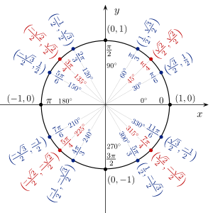
単位円とサイン・コサインの値(x軸:cos,y軸:sin)
三角関数の公式(さんかくかんすうのこうしき)は、角度に関わらず成り立つ三角関数の恒等式である。
この記事内で、角は原則として α, β, γ, θ といったギリシア文字か、x を使用する。
角度の単位としては原則としてラジアン (rad, 通常単位は省略) を用いるが、度 (°) を用いる場合もある。
- 1周 = 360度 = 2πラジアン
主な角度の度とラジアンの値は以下のようになる:
度数法(°)
|
30° |
60° |
120° |
150°
|
210° |
240° |
300° |
330°
|
弧度法(ラジアン)
|
![{\displaystyle {\frac {\pi }{6}}\!}](https://wikimedia.org/api/rest_v1/media/math/render/svg/e43048a4c319822a5aca8b56630fb16e4bf174f4) |
![{\displaystyle {\frac {\pi }{3}}\!}](https://wikimedia.org/api/rest_v1/media/math/render/svg/edda688f4310891bccb75312bad329d69d951079) |
![{\displaystyle {\frac {2\pi }{3}}\!}](https://wikimedia.org/api/rest_v1/media/math/render/svg/80bedf553ab4aa10c8bf2c3446dade44b2bdd9ce) |
|
![{\displaystyle {\frac {7\pi }{6}}\!}](https://wikimedia.org/api/rest_v1/media/math/render/svg/57d47af6f752b695071d0730329f9fc813e52315) |
![{\displaystyle {\frac {4\pi }{3}}\!}](https://wikimedia.org/api/rest_v1/media/math/render/svg/5c317c3cbd60316b1dc8bb88eedb10a4f5e3fd28) |
![{\displaystyle {\frac {5\pi }{3}}\!}](https://wikimedia.org/api/rest_v1/media/math/render/svg/983445e5b19396d4ad668c7ae30b20b3db5294b8) |
|
|
度数法(°)
|
45° |
90° |
135° |
180°
|
225° |
270° |
315° |
360°
|
弧度法(ラジアン)
|
![{\displaystyle {\frac {\pi }{4}}\!}](https://wikimedia.org/api/rest_v1/media/math/render/svg/53bc00ad36ef3da5c9554e16069da5ff87bc6799) |
![{\displaystyle {\frac {\pi }{2}}\!}](https://wikimedia.org/api/rest_v1/media/math/render/svg/bfcbc5971c250348400e43abed81abb0627fc629) |
![{\displaystyle {\frac {3\pi }{4}}\!}](https://wikimedia.org/api/rest_v1/media/math/render/svg/31b41877e3f1227eca6fafb51a3fd69b159dd866) |
|
![{\displaystyle {\frac {5\pi }{4}}\!}](https://wikimedia.org/api/rest_v1/media/math/render/svg/5abc778b053941af7082340c1d7fbbfb450f7433) |
![{\displaystyle {\frac {3\pi }{2}}\!}](https://wikimedia.org/api/rest_v1/media/math/render/svg/949828d636d75607838c594edb16b4471ce7af42) |
![{\displaystyle {\frac {7\pi }{4}}\!}](https://wikimedia.org/api/rest_v1/media/math/render/svg/72e3b5c80cba93ee8802d86d793bc2ea65468111) |
|
記事内では主にラジアンを使用し、度の場合には別記するか度を示す記号(°)を付記する。
最も基本的な関数は正弦関数(サイン、sine)と余弦関数(コサイン、cosine)である。これらは sin(θ), cos(θ) または括弧を略して sin θ, cos θ と記述される(θ は対象となる角の大きさ)。
正弦関数と余弦関数の比を正接関数(タンジェント、tangent)と言い、具体的には以下の式で表される:
![{\displaystyle \tan \theta ={\frac {\sin \theta }{\cos \theta }}}](https://wikimedia.org/api/rest_v1/media/math/render/svg/6c1226e1d3fcd47c7692602e6cbd7769db4296fe)
上記3関数の逆数関数を余割関数(コセカント、cosecant)・正割関数(セカント、secant)・余接関数(コタンジェント、cotangent)と言う。余割関数の略称には cosec と csc の2種類があり、この記事では csc を使用する。
![{\displaystyle \sec \theta ={\frac {1}{\cos \theta }},\quad \csc \theta ={\frac {1}{\sin \theta }},\quad \cot \theta ={\frac {1}{\tan \theta }}={\frac {\cos \theta }{\sin \theta }}.}](https://wikimedia.org/api/rest_v1/media/math/render/svg/e72aaa550d6c0b77be65429fcee35489c8515817)
三角関数の逆関数を逆三角関数と言う。日本語においては逆正弦関数のように頭に「逆」を付けて呼ぶ。式中では sin−1 のように右肩に "−1" を付けるか asin, arcsin のように "a" または "arc" を付ける。このarcは弧という意味がある。
この記事では逆関数として以下の表記を採用する:
関数
|
sin
|
cos
|
tan
|
sec
|
csc
|
cot
|
逆関数
|
arcsin
|
arccos
|
arctan
|
arcsec
|
arccsc
|
arccot
|
三角関数は周期関数なので、逆関数は多価関数である。
逆関数の性質から以下が成り立つ:
![{\displaystyle \sin(\arcsin x)=x,\!}](https://wikimedia.org/api/rest_v1/media/math/render/svg/c298d9103789cefb9ea2a3415b061aab16cb06e4)
![{\displaystyle \arcsin(\sin \theta )=\theta \quad {\text{for }}-\pi /2\leq \theta \leq \pi /2.}](https://wikimedia.org/api/rest_v1/media/math/render/svg/8f016fa07c595e7a820ce39bf37a4e01131399f4)
いくつかの数学記号は中等教育の課程(中学校の課程・高等学校の課程・中等教育学校の課程など)で紹介されていないため、詳しくは数学記号の表#代数学の記号など参照のこと。
ピタゴラスの定理やオイラーの公式などから以下の基本的な関係が導ける[1]。
![{\displaystyle \cos ^{2}\theta +\sin ^{2}\theta =1\!}](https://wikimedia.org/api/rest_v1/media/math/render/svg/d289030d6837455798e0cd598c565247ac26971a)
ここで sin2 θ は (sin(θ))2 を意味する。
この式を変形して、以下の式が導かれる:
![{\displaystyle \sin \theta =\pm {\sqrt {1-\cos ^{2}\theta }}}](https://wikimedia.org/api/rest_v1/media/math/render/svg/d2f68cc50a120abca6422a330a4ebc6fd0ad81c5)
![{\displaystyle \cos \theta =\pm {\sqrt {1-\sin ^{2}\theta }}}](https://wikimedia.org/api/rest_v1/media/math/render/svg/d7fb09ff408be9328891200a8898a7a1faaa9dee)
上の関係式を cos2 θ と sin2 θ で割ると、以下の関係式ができる:
![{\displaystyle 1+\tan ^{2}\theta =\sec ^{2}\theta \!}](https://wikimedia.org/api/rest_v1/media/math/render/svg/bdb7e79042cee88af0c2d9b7b0340ab5b94b0235)
![{\displaystyle 1+\cot ^{2}\theta =\csc ^{2}\theta \!}](https://wikimedia.org/api/rest_v1/media/math/render/svg/7972adaa13315fd3381ad13df9f9c9c99a02d66b)
これらの式から以下の関係を得る:
他の5種類の関数による表現[2]
|
|
|
|
|
|
|
|
|
|
|
|
|
|
|
|
|
|
|
|
|
|
|
|
|
|
|
|
|
|
|
|
|
|
|
|
|
|
|
|
|
|
|
|
|
|
|
|
|
単位円と角 θ に対する三角関数の関係。
三角関数から求められる versine, coversine, haversine, exsecant などの各関数は、かつて測量などに用いられた。例えば haversine は球面上の2点の距離を求めるのに使用された。haversineを使用すると関数表の表をひく回数を減らすことができるからである。 (参考:球面三角法) 今日ではコンピュータの発達により、これらの関数はほとんど使用されない。
versine と coversine は日本語では「正矢」「余矢」と呼ばれ、三角関数とともに八線表として1つの数表にまとめられていた。
名前
|
表記
|
値
|
versed sine, versine 正矢
|
![{\displaystyle \operatorname {versin} \theta }](https://wikimedia.org/api/rest_v1/media/math/render/svg/127e743f69b0f3ab40c96e9d4cdaba5f196f0b95)
![{\displaystyle \operatorname {vers} \theta }](https://wikimedia.org/api/rest_v1/media/math/render/svg/8323d244b596454c1cb660e976b2c11907dff76a)
|
|
versed cosine, vercosine
|
|
|
coversed sine, coversine 余矢
|
![{\displaystyle \operatorname {coversin} \theta }](https://wikimedia.org/api/rest_v1/media/math/render/svg/fd0b7aa4ccb4aabd27732c63ba5cab951dc88956)
|
|
coversed cosine, covercosine
|
|
|
half versed sine, haversine
|
|
|
half versed cosine, havercosine
|
|
|
half coversed sine, hacoversine cohaversine
|
|
|
half coversed cosine, hacovercosine cohavercosine
|
|
|
exterior secant, exsecant
|
|
|
exterior cosecant, excosecant
|
|
|
chord (弦の長さ)
|
|
|
単位円と三角関数の関係を検討することにより、以下の性質が導かれる。
いくつかの線に対し対称な図形を考えることにより、以下の関係式を得ることができる。
(x軸)に対して対称
|
(直線 y=x)に対して対称 (co- が付く関数との関係)
|
(y軸)に対して対称
|
|
|
|
単位円の図を回転させることにより、別の関係が得られる。π/2 の回転だとすべての関数が別の関数との関係を得られる。π または 2π の回転だと、同じ関数内での関係となる。
π/2 の移動
|
π の移動 tan と cot の周期
|
2π の移動 sin, cos, csc, sec の周期
|
|
|
|
以下の式は「加法定理」として知られる。これらの式は、10世紀のペルシャの数学者アブル・ワファーによって最初に示された。これらの式はオイラーの公式を用いて示すことが可能である。
Sine
|
[3]
|
Cosine
|
[3]
|
Tangent
|
[3]
|
Arcsine
|
|
Arccosine
|
|
Arctangent
|
|
上記の表において複号は同順とする。
加法定理によって、回転行列同士の積をまとめることができる。
![{\displaystyle {\begin{aligned}&{}\quad \left({\begin{array}{rr}\cos \phi &-\sin \phi \\\sin \phi &\cos \phi \end{array}}\right)\left({\begin{array}{rr}\cos \theta &-\sin \theta \\\sin \theta &\cos \theta \end{array}}\right)\\[12pt]&=\left({\begin{array}{rr}\cos \phi \cos \theta -\sin \phi \sin \theta &-\cos \phi \sin \theta -\sin \phi \cos \theta \\\sin \phi \cos \theta +\cos \phi \sin \theta &-\sin \phi \sin \theta +\cos \phi \cos \theta \end{array}}\right)\\[12pt]&=\left({\begin{array}{rr}\cos(\theta +\phi )&-\sin(\theta +\phi )\\\sin(\theta +\phi )&\cos(\theta +\phi )\end{array}}\right)\end{aligned}}}](https://wikimedia.org/api/rest_v1/media/math/render/svg/852d1e76b4190362dde8aefd41ddca69347d1961)
正弦関数と余弦関数において、以下の式が成り立つ。
![{\displaystyle \sin \left(\sum _{i=1}^{\infty }\theta _{i}\right)=\sum _{{\text{odd}}\ k\geq 1}(-1)^{(k-1)/2}\sum _{\begin{smallmatrix}A\subseteq \{\,1,2,3,\dots \,\}\\\left|A\right|=k\end{smallmatrix}}\left(\prod _{i\in A}\sin \theta _{i}\prod _{i\not \in A}\cos \theta _{i}\right)}](https://wikimedia.org/api/rest_v1/media/math/render/svg/441ded49a9ad0e60f4454da098e8cc1ea7c983f3)
![{\displaystyle \cos \left(\sum _{i=1}^{\infty }\theta _{i}\right)=\sum _{{\text{even}}\ k\geq 0}~(-1)^{k/2}~~\sum _{\begin{smallmatrix}A\subseteq \{\,1,2,3,\dots \,\}\\\left|A\right|=k\end{smallmatrix}}\left(\prod _{i\in A}\sin \theta _{i}\prod _{i\not \in A}\cos \theta _{i}\right)}](https://wikimedia.org/api/rest_v1/media/math/render/svg/e3496a329a142adb4a327a0f904e80b4799ffb41)
いずれの場合にも、「有限個の角の正弦関数と残りの角の余弦関数の積」の和となる。無限の和に見えるが、j 以上のすべての i で θi=0 が成り立つ場合、j 以上の k は計算する必要がなく有限項の計算となる。
ek (k ∈ {0, ..., n}) を k次の基本対称式とする。
![{\displaystyle x_{i}=\tan \theta _{i}\,}](https://wikimedia.org/api/rest_v1/media/math/render/svg/d4c2557b3dfbdbf0514cb927c755a57ad8da86ce)
のとき i ∈ {0, ..., n} に対して以下のようになる。
![{\displaystyle {\begin{aligned}e_{0}&=1\\[6pt]e_{1}&=\sum _{1\leq i\leq n}x_{i}&&=\sum _{1\leq i\leq n}\tan \theta _{i}\\[6pt]e_{2}&=\sum _{1\leq i<j\leq n}x_{i}x_{j}&&=\sum _{1\leq i<j\leq n}\tan \theta _{i}\tan \theta _{j}\\[6pt]e_{3}&=\sum _{1\leq i<j<k\leq n}x_{i}x_{j}x_{k}&&=\sum _{1\leq i<j<k\leq n}\tan \theta _{i}\tan \theta _{j}\tan \theta _{k}\\&{}\ \ \vdots &&{}\ \ \vdots \end{aligned}}}](https://wikimedia.org/api/rest_v1/media/math/render/svg/9a1d7a75d1ce780643b0b3bc40f9ad3c03ed2b44)
このとき正接関数の和は以下の式で表される。
![{\displaystyle \tan(\theta _{1}+\cdots +\theta _{n})={\frac {e_{1}-e_{3}+e_{5}-\cdots }{e_{0}-e_{2}+e_{4}-\cdots }},\!}](https://wikimedia.org/api/rest_v1/media/math/render/svg/89ac58204934f8506f8043e11e0a9ed6b50e63ad)
この e は、en まで使用する。
例
![{\displaystyle {\begin{aligned}\tan(\theta _{1}+\theta _{2})&={\frac {e_{1}}{e_{0}-e_{2}}}={\frac {x_{1}+x_{2}}{1\ -\ x_{1}x_{2}}}={\frac {\tan \theta _{1}+\tan \theta _{2}}{1\ -\ \tan \theta _{1}\tan \theta _{2}}},\\\\\tan(\theta _{1}+\theta _{2}+\theta _{3})&={\frac {e_{1}-e_{3}}{e_{0}-e_{2}}}={\frac {(x_{1}+x_{2}+x_{3})\ -\ (x_{1}x_{2}x_{3})}{1\ -\ (x_{1}x_{2}+x_{1}x_{3}+x_{2}x_{3})}},\\\\\tan(\theta _{1}+\theta _{2}+\theta _{3}+\theta _{4})&={\frac {e_{1}-e_{3}}{e_{0}-e_{2}+e_{4}}}\\\\&={\frac {(x_{1}+x_{2}+x_{3}+x_{4})\ -\ (x_{1}x_{2}x_{3}+x_{1}x_{2}x_{4}+x_{1}x_{3}x_{4}+x_{2}x_{3}x_{4})}{1\ -\ (x_{1}x_{2}+x_{1}x_{3}+x_{1}x_{4}+x_{2}x_{3}+x_{2}x_{4}+x_{3}x_{4})\ +\ (x_{1}x_{2}x_{3}x_{4})}},\end{aligned}}}](https://wikimedia.org/api/rest_v1/media/math/render/svg/ae745b59fce5aeae2126a2f25f1ff6d62783f879)
数学的帰納法を用いて証明が可能である。
ek は前節同様正接関数の基本対称式とする。
![{\displaystyle {\begin{aligned}\sec(\theta _{1}+\cdots +\theta _{n})&={\frac {\sec \theta _{1}\cdots \sec \theta _{n}}{e_{0}-e_{2}+e_{4}-\cdots }}\\[8pt]\csc(\theta _{1}+\cdots +\theta _{n})&={\frac {\sec \theta _{1}\cdots \sec \theta _{n}}{e_{1}-e_{3}+e_{5}-\cdots }}\end{aligned}}}](https://wikimedia.org/api/rest_v1/media/math/render/svg/2c82ca2d8da55d938d78aad99295a11f79665fde)
例
![{\displaystyle {\begin{aligned}\sec(\alpha +\beta +\gamma )&={\frac {\sec \alpha \sec \beta \sec \gamma }{1-\tan \alpha \tan \beta -\tan \alpha \tan \gamma -\tan \beta \tan \gamma }}\\[8pt]\csc(\alpha +\beta +\gamma )&={\frac {\sec \alpha \sec \beta \sec \gamma }{\tan \alpha +\tan \beta +\tan \gamma -\tan \alpha \tan \beta \tan \gamma }}\end{aligned}}}](https://wikimedia.org/api/rest_v1/media/math/render/svg/932e894ff60465fb368b7d6fceb7977d53c2739b)
Tn は n 次のチェビシェフ多項式
|
[4]
|
Sn は n 次の spread 多項式
|
|
ド・モアブルの定理による(i は虚数単位)
|
|
ディリクレ核
|
|
以下の式は加法定理などから容易に導くことができる。
倍角[5]
|
|
|
|
|
三倍角[4]
|
|
|
|
|
半角[6]
|
|
|
|
|
正弦関数と余弦関数の三倍角の公式は、元の関数の三次方程式で表すことができる。従って、三次方程式の解を求めることでそれらの三角関数の値を得ることができる。
幾何学的には、三倍角の公式を経由し三角関数の値を求めることは角の三等分問題に相当する。この問題は、定規とコンパスを用いた解法が特別な角を除いて存在しないことが知られている。
方程式 x3 − 3x + d/4 = 0(正弦関数ならば x = sinθ, d = sin(3θ) とする)の判別式は正なのでこの方程式は3つの実数解を持つ。
加法定理から、正弦関数および余弦関数の以下の倍角公式が得られる。これらの式は16世紀のフランスの数学者フランソワ・ビエトによって示された。
![{\displaystyle {\begin{aligned}\sin(n\theta )&=\sum _{k=0}^{n}{\binom {n}{k}}\cos ^{k}\theta \,\sin ^{n-k}\theta \,\sin \left({\frac {1}{2}}(n-k)\pi \right),\\\cos(n\theta )&=\sum _{k=0}^{n}{\binom {n}{k}}\cos ^{k}\theta \,\sin ^{n-k}\theta \,\cos \left({\frac {1}{2}}(n-k)\pi \right)\end{aligned}}}](https://wikimedia.org/api/rest_v1/media/math/render/svg/954cdb1e30f603715b36e02c8892285875386ee5)
ここで (n
k) は二項係数である。上記の和の最初の数項を明示すれば、以下の通りである。
![{\displaystyle {\begin{aligned}\sin(n\theta )&={\binom {n}{1}}\cos ^{n-1}\theta \sin \theta -{\binom {n}{3}}\cos ^{n-3}\theta \sin ^{3}\theta +\cdots ,\\\cos(n\theta )&={\binom {n}{0}}\cos ^{n}\theta -{\binom {n}{2}}\cos ^{n-2}\theta \sin ^{2}\theta +\cdots .\end{aligned}}}](https://wikimedia.org/api/rest_v1/media/math/render/svg/1390318e478140a241357014c2248fe42304281f)
ビエトの公式を利用し、正接関数と余接関数の倍角公式を漸化式として与えることができる。
![{\displaystyle {\begin{aligned}\tan {((n+1)\theta )}&={\frac {\tan(n\theta )+\tan \theta }{1-\tan(n\theta )\tan \theta }},\\\cot {((n+1)\theta )}&={\frac {\cot(n\theta )\cot \theta -1}{\cot {(n\theta )}+\cot \theta }}.\end{aligned}}}](https://wikimedia.org/api/rest_v1/media/math/render/svg/aa2d75714cc3fc779015e7e1ff133d967b5e82eb)
またド・モアブルの定理、あるいはオイラーの公式を利用し、以下のように表すことができる。
![{\displaystyle {\begin{aligned}\cos(n\theta )&={\frac {1}{2}}\left\{(\cos \theta +i\sin \theta )^{n}+(\cos \theta -i\sin \theta )^{n}\right\},\\\sin(n\theta )&=-{\frac {i}{2}}\left\{(\cos \theta +i\sin \theta )^{n}-(\cos \theta -i\sin \theta )^{n}\right\},\\\tan(n\theta )&=-i{\frac {(1+i\tan \theta )^{n}-(1-i\tan \theta )^{n}}{(1+i\tan \theta )^{n}+(1-i\tan \theta )^{n}}}\end{aligned}}}](https://wikimedia.org/api/rest_v1/media/math/render/svg/fde15c62da8ad40d040363db8c768e643840242d)
パフヌティ・チェビシェフは、n 倍角の正弦関数と余弦関数の値を、(n − 1) 倍角と (n − 2) 倍角の値を用いて表す方法を発見している[7]。
cos(nx) は、以下のように表される。
![{\displaystyle \cos(nx)=2\cdot \cos x\cdot \cos((n-1)x)-\cos((n-2)x)\,}](https://wikimedia.org/api/rest_v1/media/math/render/svg/7c5115dfacf4c0dce2f76cfedefa4d9d53ead7eb)
同様に sin(nx) は以下のように表される。
![{\displaystyle \sin(nx)=2\cdot \cos x\cdot \sin((n-1)x)-\sin((n-2)x)\,}](https://wikimedia.org/api/rest_v1/media/math/render/svg/6492660300bfe0f5c0d116f229fddc6bd6edf224)
tan(nx) は以下のようになる。
![{\displaystyle \tan(nx)={\frac {H+K\tan x}{K-H\tan x}}\,}](https://wikimedia.org/api/rest_v1/media/math/render/svg/b9b4595c1030478d3a91970507197804c86270d6)
ここで、H/K = tan((n − 1)x) である。
α, β の算術平均の正接について以下が成り立つ。
![{\displaystyle \tan \left({\frac {\alpha +\beta }{2}}\right)={\frac {\sin \alpha +\sin \beta }{\cos \alpha +\cos \beta }}=-\,{\frac {\cos \alpha -\cos \beta }{\sin \alpha -\sin \beta }}}](https://wikimedia.org/api/rest_v1/media/math/render/svg/e0059ec572ecb7f76446d6d49406212189d349cf)
α, β のいずれかが 0 である場合、これは正接関数の半角公式に一致する。
以下の式が成り立つ。
![{\displaystyle \cos \left({\theta \over 2}\right)\cdot \cos \left({\theta \over 4}\right)\cdot \cos \left({\theta \over 8}\right)\cdots =\prod _{n=1}^{\infty }\cos \left({\theta \over 2^{n}}\right)={\sin(\theta ) \over \theta }=\operatorname {sinc} \,\theta .}](https://wikimedia.org/api/rest_v1/media/math/render/svg/9ada3e54df23601cc6b6861a1ea9eefece1ea35e)
最後のsincは、正弦関数を角の大きさで割ったものである。
![{\displaystyle \operatorname {sinc} x:={\frac {\sin x}{x}}.}](https://wikimedia.org/api/rest_v1/media/math/render/svg/b0cd99caf251970eb0517666d210573b06337c4f)
余弦関数の倍角公式を変形することにより、以下の式が得られる。式の次数を下げるためによく用いられる。
正弦関数
|
余弦関数
|
その他
|
|
|
|
|
|
|
|
|
|
|
|
|
ド・モアブルの定理・オイラーの公式・二項定理を用いると、以下のように一般化できる。
|
余弦関数
|
正弦関数
|
n が奇数
|
|
|
n が偶数
|
|
|
加法定理に(θ±φ)を代入することにより、積和公式を導くことができる。これを変形すると和積公式になる。
積和公式
|
|
|
|
|
|
和積公式
|
|
|
|
|
シャルル・エルミートは、複素関数に関する以下の式を示した。
複素数 a1, ..., an は、どの2つをとってもその差がπの整数倍にならないものとする。
![{\displaystyle A_{n,k}=\prod _{\begin{smallmatrix}1\leq j\leq n\\j\neq k\end{smallmatrix}}\cot(a_{k}-a_{j})}](https://wikimedia.org/api/rest_v1/media/math/render/svg/add4d3e70d16463f3a6941af196afc1e6c337ad1)
と置く(A1,1 のときこの値は1とする)と、以下の式が成り立つ。
![{\displaystyle \cot(z-a_{1})\cdots \cot(z-a_{n})=\cos {\frac {n\pi }{2}}+\sum _{k=1}^{n}A_{n,k}\cot(z-a_{k}).}](https://wikimedia.org/api/rest_v1/media/math/render/svg/9db60873e93178b3b00e9cdea04ca45727748be1)
自明でない単純な例として、n = 2 のときの例をあげる。
![{\displaystyle \cot(z-a_{1})\cot(z-a_{2})=-1+\cot(a_{1}-a_{2})\cot(z-a_{1})+\cot(a_{2}-a_{1})\cot(z-a_{2})}](https://wikimedia.org/api/rest_v1/media/math/render/svg/7a4abdd500af44fa79f98f4d643391ca19d544a1)
正弦関数と余弦関数の和は、正弦関数で表すことができる。
![{\displaystyle a\sin x+b\cos x={\sqrt {a^{2}+b^{2}}}\cdot \sin(x+\varphi )\,}](https://wikimedia.org/api/rest_v1/media/math/render/svg/122a9fdc91f13be1d551abbc0275c26956b48b2e)
ここで、φの値は以下の式で与えられる。
![{\displaystyle \varphi ={\begin{cases}\arcsin \left({\frac {b}{\sqrt {a^{2}+b^{2}}}}\right)&{\text{if }}a\geq 0,\\\pi -\arcsin \left({\frac {b}{\sqrt {a^{2}+b^{2}}}}\right)&{\text{if }}a<0,\end{cases}}}](https://wikimedia.org/api/rest_v1/media/math/render/svg/84827dff78a11559eaada73ce202b1cb4d0a168f)
または
![{\displaystyle \varphi =\arctan \left({\frac {b}{a}}\right)+{\begin{cases}0&{\text{if }}a\geq 0,\\\pi &{\text{if }}a<0,\end{cases}}}](https://wikimedia.org/api/rest_v1/media/math/render/svg/663426c495d325fa51e914026ec1730ff1c44a79)
位相の違う正弦関数を以下のように合成することができる。
![{\displaystyle a\sin x+b\sin(x+\alpha )=c\sin(x+\beta )\,}](https://wikimedia.org/api/rest_v1/media/math/render/svg/84311711d59b3dcb5695c94cf7d5c1a625054270)
ここで c と β の値は以下の式で与えられる。
![{\displaystyle c={\sqrt {a^{2}+b^{2}+2ab\cos \alpha }},\,}](https://wikimedia.org/api/rest_v1/media/math/render/svg/b08f61d3442a3ea48c3657a706a5ec6a5e548e6a)
![{\displaystyle \beta =\arctan \left({\frac {b\sin \alpha }{a+b\cos \alpha }}\right)+{\begin{cases}0&{\text{if }}a+b\cos \alpha \geq 0,\\\pi &{\text{if }}a+b\cos \alpha <0.\end{cases}}}](https://wikimedia.org/api/rest_v1/media/math/render/svg/718c29df64d7a0135dc30188746fcdb197a39947)
正弦関数と余弦関数の和に関する以下のような公式がある[8]。
![{\displaystyle {\begin{aligned}&\sin {\varphi }+\sin {(\varphi +\alpha )}+\sin {(\varphi +2\alpha )}+\cdots {}\\[8pt]&{}\qquad \qquad \cdots +\sin {(\varphi +n\alpha )}={\frac {\sin {\left({\frac {(n+1)\alpha }{2}}\right)}\cdot \sin {(\varphi +{\frac {n\alpha }{2}})}}{\sin {\frac {\alpha }{2}}}}.\\[10pt]&\cos {\varphi }+\cos {(\varphi +\alpha )}+\cos {(\varphi +2\alpha )}+\cdots {}\\[8pt]&{}\qquad \qquad \cdots +\cos {(\varphi +n\alpha )}={\frac {\sin {\left({\frac {(n+1)\alpha }{2}}\right)}\cdot \cos {(\varphi +{\frac {n\alpha }{2}})}}{\sin {\frac {\alpha }{2}}}}.\end{aligned}}}](https://wikimedia.org/api/rest_v1/media/math/render/svg/cf3414d47dcb384f6ef6779a03fc3f6bf78c2277)
正接関数と正割関数に関して以下の式が成り立つ。
![{\displaystyle \tan x+\sec x=\tan \left({x \over 2}+{\pi \over 4}\right)=\exp \left(\operatorname {gd} ^{-1}x\right)}](https://wikimedia.org/api/rest_v1/media/math/render/svg/3e39b6309cb4a2463bbcb57ad87220cadede6439)
ただし、
はグーデルマン関数の逆関数である。
ƒ(x) と g(x) を以下のようなメビウス変換関数として定義する。
![{\displaystyle f(x)={\frac {(\cos \alpha )x-\sin \alpha }{(\sin \alpha )x+\cos \alpha }},}](https://wikimedia.org/api/rest_v1/media/math/render/svg/cbc62585cae3c00794e045d021d6bb010afee79b)
![{\displaystyle g(x)={\frac {(\cos \beta )x-\sin \beta }{(\sin \beta )x+\cos \beta }},}](https://wikimedia.org/api/rest_v1/media/math/render/svg/dd4ca80eca844d6808928b5c9c6bbfeec9d09f53)
このとき以下が成り立つ。
![{\displaystyle f(g(x))=g(f(x))={\frac {(\cos(\alpha +\beta ))x-\sin(\alpha +\beta )}{(\sin(\alpha +\beta ))x+\cos(\alpha +\beta )}}.}](https://wikimedia.org/api/rest_v1/media/math/render/svg/9d8f99d1ad8776fffb1246c7429243819022cbe3)
以下のように書くこともできる。
![{\displaystyle f_{\alpha }\circ f_{\beta }=f_{\alpha +\beta }.\,}](https://wikimedia.org/api/rest_v1/media/math/render/svg/c0e9bfaa32426a4ca6be9241b995716867550771)
![{\displaystyle \arcsin x+\arccos x={\frac {\pi }{2}}}](https://wikimedia.org/api/rest_v1/media/math/render/svg/71bece6bfb4361d44a5220e9eec101598ad03195)
![{\displaystyle \arctan x+\operatorname {arccot} x={\frac {\pi }{2}}.}](https://wikimedia.org/api/rest_v1/media/math/render/svg/81469b2545052eaaf39b22e983dbcbfb5f09eb99)
![{\displaystyle \arctan x+\arctan {\frac {1}{x}}=\left\{{\begin{matrix}{\frac {\pi }{2}},&{\mbox{if }}x>0\\-{\frac {\pi }{2}},&{\mbox{if }}x<0\end{matrix}}\right.}](https://wikimedia.org/api/rest_v1/media/math/render/svg/aabac1ced39ee68830ff3f22887f23e06ae5f927)
|
arccos
|
arcsin
|
arctan
|
arccot
|
arccos
|
|
|
|
|
arcsin
|
|
|
|
|
arctan
|
|
|
|
|
arccot
|
|
|
|
|
式
|
和
|
条件
|
|
|
または
|
|
|
かつ かつ
|
|
|
かつ かつ
|
|
|
または
|
|
|
かつ かつ
|
|
|
かつ かつ
|
|
|
|
|
|
|
|
|
|
|
|
|
|
|
|
|
|
かつ
|
|
|
かつ
|
|
|
|
|
|
かつ
|
|
|
かつ
|
|
|
|
|
|
|
|
|
以下において、
は虚数単位とする。
(オイラーの公式)
![{\displaystyle e^{-ix}=\cos(-x)+i\sin(-x)=\cos(x)-i\sin(x)}](https://wikimedia.org/api/rest_v1/media/math/render/svg/d9114531f66938479e7ce6315fa492b5fdcb844f)
(オイラーの等式)
![{\displaystyle \cos(x)={\frac {e^{ix}+e^{-ix}}{2}}\;}](https://wikimedia.org/api/rest_v1/media/math/render/svg/c8f52446887052c87511159b7b8113f3bc4cb092)
![{\displaystyle \sin(x)={\frac {e^{ix}-e^{-ix}}{2i}}\;}](https://wikimedia.org/api/rest_v1/media/math/render/svg/524466c42d884cea2a537eaa9e29eec04431381b)
![{\displaystyle \tan(x)={\frac {e^{ix}-e^{-ix}}{i({e^{ix}+e^{-ix}})}}\;={\frac {\sin(x)}{\cos(x)}}}](https://wikimedia.org/api/rest_v1/media/math/render/svg/95d788e523e5f3fd4c34b094564f2968ee65864d)
いくつかの関数は、無限乗積の形で表すことができる。
は総乗を示す。
α, β, γ が三角形の3つの角の大きさのとき、即ち α + β + γ = π を満たす場合、以下の式が成り立つ。
![{\displaystyle \tan \alpha +\tan \beta +\tan \gamma =\tan \alpha \cdot \tan \beta \cdot \tan \gamma \,}](https://wikimedia.org/api/rest_v1/media/math/render/svg/0fe8c152093098d464f496dd0de3913f1529ca86)
![{\displaystyle \cot \beta \cdot \cot \gamma +\cot \gamma \cdot \cot \alpha +\cot \alpha \cdot \cot \beta =1}](https://wikimedia.org/api/rest_v1/media/math/render/svg/74fcc3c197ed624c70b6cfc00746cb2ef548c046)
![{\displaystyle \cot {\frac {\alpha }{2}}+\cot {\frac {\beta }{2}}+\cot {\frac {\gamma }{2}}=\cot {\frac {\alpha }{2}}\cdot \cot {\frac {\beta }{2}}\cdot \cot {\frac {\gamma }{2}}}](https://wikimedia.org/api/rest_v1/media/math/render/svg/a62b0958247ab0e8f1bc729f2678941a1addedc1)
![{\displaystyle \tan {\frac {\beta }{2}}\tan {\frac {\gamma }{2}}+\tan {\frac {\gamma }{2}}\tan {\frac {\alpha }{2}}+\tan {\frac {\alpha }{2}}\tan {\frac {\beta }{2}}=1}](https://wikimedia.org/api/rest_v1/media/math/render/svg/aca762a805db0c80b84d38043a0de29a702f45f1)
![{\displaystyle \sin \alpha +\sin \beta +\sin \gamma =4\cos {\frac {\alpha }{2}}\cos {\frac {\beta }{2}}\cos {\frac {\gamma }{2}}}](https://wikimedia.org/api/rest_v1/media/math/render/svg/78731cad789eccabfe272fc5d2a85dbd1c044da6)
![{\displaystyle -\sin \alpha +\sin \beta +\sin \gamma =4\cos {\frac {\alpha }{2}}\sin {\frac {\beta }{2}}\sin {\frac {\gamma }{2}}}](https://wikimedia.org/api/rest_v1/media/math/render/svg/512cb66b272c60f4339f2d55f794701a44fe3e6c)
![{\displaystyle \cos \alpha +\cos \beta +\cos \gamma =4\sin {\frac {\alpha }{2}}\sin {\frac {\beta }{2}}\sin {\frac {\gamma }{2}}+1}](https://wikimedia.org/api/rest_v1/media/math/render/svg/9a518b4be27361bd289667bee5e7305ba8789336)
![{\displaystyle -\cos \alpha +\cos \beta +\cos \gamma =4\sin {\frac {\alpha }{2}}\cos {\frac {\beta }{2}}\cos {\frac {\gamma }{2}}-1}](https://wikimedia.org/api/rest_v1/media/math/render/svg/43a71ae15010ea24ecb46d8e389a1b48b4a232a3)
![{\displaystyle \sin(2\alpha )+\sin(2\beta )+\sin(2\gamma )=4\sin \alpha \sin \beta \sin \gamma \,}](https://wikimedia.org/api/rest_v1/media/math/render/svg/8a182dc8e41c5ed26d6052afd54b6102798c24a2)
![{\displaystyle -\sin(2\alpha )+\sin(2\beta )+\sin(2\gamma )=4\sin \alpha \cos \beta \cos \gamma \,}](https://wikimedia.org/api/rest_v1/media/math/render/svg/f1303150422913d46b79007810ec83ec04d7492d)
![{\displaystyle \cos(2\alpha )+\cos(2\beta )+\cos(2\gamma )=-4\cos \alpha \cos \beta \cos \gamma -1\,}](https://wikimedia.org/api/rest_v1/media/math/render/svg/a99709f9455d580927fb04d03257d661f56478b0)
![{\displaystyle -\cos(2\alpha )+\cos(2\beta )+\cos(2\gamma )=-4\cos \alpha \sin \beta \sin \gamma +1\,}](https://wikimedia.org/api/rest_v1/media/math/render/svg/af536d5481f5c224827712919ca39242ddb9f9d7)
![{\displaystyle \sin ^{2}\alpha +\sin ^{2}\beta +\sin ^{2}\gamma =2\cos \alpha \cos \beta \cos \gamma +2\,}](https://wikimedia.org/api/rest_v1/media/math/render/svg/cf4594072223ea59dfe0523199f1f95f4850b07f)
![{\displaystyle -\sin ^{2}\alpha +\sin ^{2}\beta +\sin ^{2}\gamma =2\cos \alpha \sin \beta \sin \gamma \,}](https://wikimedia.org/api/rest_v1/media/math/render/svg/5cb3387b0b44b7aea23e504cbc98c305e880b421)
![{\displaystyle \cos ^{2}\alpha +\cos ^{2}\beta +\cos ^{2}\gamma =-2\cos \alpha \cos \beta \cos \gamma +1\,}](https://wikimedia.org/api/rest_v1/media/math/render/svg/ec0ec88839c3ce21a1029f3c21681d581572a49e)
![{\displaystyle -\cos ^{2}\alpha +\cos ^{2}\beta +\cos ^{2}\gamma =-2\cos \alpha \sin \beta \sin \gamma +1\,}](https://wikimedia.org/api/rest_v1/media/math/render/svg/7580566f8218c0e390a62c2743b5863a82ab668b)
![{\displaystyle \sin ^{2}(2\alpha )+\sin ^{2}(2\beta )+\sin ^{2}(2\gamma )=-2\cos(2\alpha )\,\cos(2\beta )\,\cos(2\gamma )+2}](https://wikimedia.org/api/rest_v1/media/math/render/svg/c0a7224aa5b44470893fff80831fb09b7e243b1b)
![{\displaystyle \cos ^{2}(2\alpha )+\cos ^{2}(2\beta )+\cos ^{2}(2\gamma )=2\cos(2\alpha )\,\cos(2\beta )\,\cos(2\gamma )+1}](https://wikimedia.org/api/rest_v1/media/math/render/svg/a9edc2c3be030b68c17e5a66bff700816edb3728)
以下の式が成り立つ。
(モリーの法則)
この式は以下の式の特殊な場合である。
![{\displaystyle \prod _{j=0}^{k-1}\cos \left(2^{j}x\right)={\frac {\sin \left(2^{k}x\right)}{2^{k}\sin(x)}}.}](https://wikimedia.org/api/rest_v1/media/math/render/svg/caf00c322084ea6a80b1fd837fadd3e846fd395a)
以下の式も同じ値を持つ。
![{\displaystyle \cos {\frac {\pi }{7}}\cos {\frac {2\pi }{7}}\cos {\frac {3\pi }{7}}={\frac {1}{8}},}](https://wikimedia.org/api/rest_v1/media/math/render/svg/227c7062e815774a127eef0ca4f331ff570c4976)
正弦関数では以下の式が成り立つ。
![{\displaystyle \sin 10^{\circ }\cdot \sin 50^{\circ }\cdot \sin 70^{\circ }={\frac {1}{8}}.}](https://wikimedia.org/api/rest_v1/media/math/render/svg/481c028cc1989226779b0fd8083f4c7ecfaaa289)
![{\displaystyle \sin 15^{\circ }\cdot \sin 75^{\circ }={\frac {1}{4}}.}](https://wikimedia.org/api/rest_v1/media/math/render/svg/2981af285400f288c3ed5ced7de0365d47a036a5)
![{\displaystyle \sin 20^{\circ }\cdot \sin 40^{\circ }\cdot \sin 80^{\circ }={\frac {\sqrt {3}}{8}}.}](https://wikimedia.org/api/rest_v1/media/math/render/svg/fe0b34fc8b4d1c4742d4b4903725fa5c48d33a08)
余弦関数では以下の式が成り立つ。
![{\displaystyle \cos 10^{\circ }\cdot \cos 50^{\circ }\cdot \cos 70^{\circ }={\frac {\sqrt {3}}{8}}.}](https://wikimedia.org/api/rest_v1/media/math/render/svg/3a40fcca60acd8a6ab20fea5ea41f58ddb9118a9)
![{\displaystyle \cos 15^{\circ }\cdot \cos 75^{\circ }={\frac {1}{4}}.}](https://wikimedia.org/api/rest_v1/media/math/render/svg/d7c489fa283280c5f06740085945de7763d04504)
上の式を利用して以下の式が得られる。
![{\displaystyle \tan 50^{\circ }+\tan 60^{\circ }+\tan 70^{\circ }=\tan 50^{\circ }\cdot \tan 60^{\circ }\cdot \tan 70^{\circ }=\tan 80^{\circ }.}](https://wikimedia.org/api/rest_v1/media/math/render/svg/446d61c0007539964ec789ca7247a2574de8d614)
以下の式は単純である。
![{\displaystyle \cos 24^{\circ }+\cos 48^{\circ }+\cos 96^{\circ }+\cos 168^{\circ }={\frac {1}{2}}.}](https://wikimedia.org/api/rest_v1/media/math/render/svg/4006eb68677ca45758bbbb6eb2a348dfe881d4c8)
上の式を一般化する場合分母に21が出てくるため、単位として度よりもラジアンを使用した方がよい。
![{\displaystyle {\begin{aligned}&\cos \left({\frac {2\pi }{21}}\right)+\cos \left(2\cdot {\frac {2\pi }{21}}\right)+\cos \left(4\cdot {\frac {2\pi }{21}}\right)\\[10pt]&{}\qquad {}+\cos \left(5\cdot {\frac {2\pi }{21}}\right)+\cos \left(8\cdot {\frac {2\pi }{21}}\right)+\cos \left(10\cdot {\frac {2\pi }{21}}\right)={\frac {1}{2}}.\end{aligned}}}](https://wikimedia.org/api/rest_v1/media/math/render/svg/15e07fe52f1162c9c933e28a6bec4fb9f59528e8)
係数に登場する 1, 2, 4, 5, 8, 10 は 21/2 より小さく 21 と互いに素な全ての自然数である。この式は円分多項式に関係している。
以下の関係から導かれる式もある。
![{\displaystyle \prod _{k=1}^{n-1}\sin \left({\frac {k\pi }{n}}\right)={\frac {n}{2^{n-1}}}}](https://wikimedia.org/api/rest_v1/media/math/render/svg/57861b2da169da4278cf0c6085dd8ffe3ffb1502)
![{\displaystyle \prod _{k=1}^{n-1}\cos \left({\frac {k\pi }{n}}\right)={\frac {\sin \left(\pi n/2\right)}{2^{n-1}}}}](https://wikimedia.org/api/rest_v1/media/math/render/svg/6ea10f89123bfc78a1f2f1d22c5f206d98231fd6)
これらを組み合わせると、以下の式になる。
![{\displaystyle \prod _{k=1}^{n-1}\tan \left({\frac {k\pi }{n}}\right)={\frac {n}{\sin \left(\pi n/2\right)}}}](https://wikimedia.org/api/rest_v1/media/math/render/svg/a5d666bf6eb9601d578f781f30912895767355a4)
n を奇数に限定すると、以下の式が得られる。
![{\displaystyle \prod _{k=1}^{m}\tan \left({\frac {k\pi }{2m+1}}\right)={\sqrt {2m+1}}}](https://wikimedia.org/api/rest_v1/media/math/render/svg/40d115c3ba55d85e172221e4d629f1eb48bda8b4)
円周率の計算において、以下のマチンの公式はよく使用される。
![{\displaystyle {\frac {\pi }{4}}=4\arctan {\frac {1}{5}}-\arctan {\frac {1}{239}}}](https://wikimedia.org/api/rest_v1/media/math/render/svg/ba362ff207097dc35ca873f9a16bcda21a96b278)
レオンハルト・オイラーは、以下の式を示している。
![{\displaystyle {\frac {\pi }{4}}=5\arctan {\frac {1}{7}}+2\arctan {\frac {3}{79}}.}](https://wikimedia.org/api/rest_v1/media/math/render/svg/c3ed05dee249464344bcae45d7b6f2b6021409e4)
正弦関数と余弦関数において、値が
(ただし 0 ≤ n ≤ 4)の形になるものは、覚えやすい値である。
![{\displaystyle {\begin{matrix}\sin 0&=&\sin 0^{\circ }&=&{\sqrt {0}}/2&=&\cos 90^{\circ }&=&\cos \left({\frac {\pi }{2}}\right)\\\\\sin \left({\frac {\pi }{6}}\right)&=&\sin 30^{\circ }&=&{\sqrt {1}}/2&=&\cos 60^{\circ }&=&\cos \left({\frac {\pi }{3}}\right)\\\\\sin \left({\frac {\pi }{4}}\right)&=&\sin 45^{\circ }&=&{\sqrt {2}}/2&=&\cos 45^{\circ }&=&\cos \left({\frac {\pi }{4}}\right)\\\\\sin \left({\frac {\pi }{3}}\right)&=&\sin 60^{\circ }&=&{\sqrt {3}}/2&=&\cos 30^{\circ }&=&\cos \left({\frac {\pi }{6}}\right)\\\\\sin \left({\frac {\pi }{2}}\right)&=&\sin 90^{\circ }&=&{\sqrt {4}}/2&=&\cos 0^{\circ }&=&\cos 0\end{matrix}}}](https://wikimedia.org/api/rest_v1/media/math/render/svg/4b428787bdd07ac594ec15f5700e8c0a050970eb)
一部の角に対する値は、黄金比 φ を用いて表すことができる。
![{\displaystyle \cos \left({\frac {\pi }{5}}\right)=\cos 36^{\circ }={{\sqrt {5}}+1 \over 4}={\frac {\varphi }{2}}}](https://wikimedia.org/api/rest_v1/media/math/render/svg/3792ef234f059ccf933d83eedee459fbd5eafc6b)
![{\displaystyle \sin \left({\frac {\pi }{10}}\right)=\sin 18^{\circ }={{\sqrt {5}}-1 \over 4}={\varphi -1 \over 2}={1 \over 2\varphi }}](https://wikimedia.org/api/rest_v1/media/math/render/svg/637ce4a172421f7f3c6b3c645d05128f2e099fe1)
ユークリッドは原論13巻で、正五角形と同じ長さの辺を持つ正方形の面積は、同じ円に内接する正六角形と正十角形の辺の長さを持つ2つの正方形の和に等しいことを示した。これを三角関数を用いて書くと以下のようになる。
![{\displaystyle \sin ^{2}{18^{\circ }}+\sin ^{2}{30^{\circ }}=\sin ^{2}{36^{\circ }}.\,}](https://wikimedia.org/api/rest_v1/media/math/render/svg/304c1952b2ad72353760b756e9fa2cc35dcfda29)
微分積分学の分野においては、角度はラジアンを使用する。
微積分において、極限に関する2つの重要な式がある。1つは
![{\displaystyle \lim _{x\rightarrow 0}{\frac {\sin x}{x}}=1,}](https://wikimedia.org/api/rest_v1/media/math/render/svg/cec799a02babc80e531aa1c085a0f9d1fafe2886)
である。この式ははさみうちの原理から導くことができる。もう1つは以下の式である。
![{\displaystyle \lim _{x\rightarrow 0}{\frac {1-\cos x}{x}}=0,}](https://wikimedia.org/api/rest_v1/media/math/render/svg/e1b6dad3145dbc7562aeb910faf6fd069860ecb1)
これらの式と加法定理などを利用して、以下の式を導くことができる。
![{\displaystyle {d \over dx}\sin x=\cos x}](https://wikimedia.org/api/rest_v1/media/math/render/svg/c976bcdb6b29573bc73f234a44acd4f9bb3ea8d3)
以下に三角関数と逆三角関数の微分を示す。
![{\displaystyle {\begin{aligned}{d \over dx}\sin x&=\cos x,&{d \over dx}\arcsin x&={1 \over {\sqrt {1-x^{2}}}}\\\\{d \over dx}\cos x&=-\sin x,&{d \over dx}\arccos x&={-1 \over {\sqrt {1-x^{2}}}}\\\\{d \over dx}\tan x&=\sec ^{2}x,&{d \over dx}\arctan x&={1 \over 1+x^{2}}\\\\{d \over dx}\cot x&=-\csc ^{2}x,&{d \over dx}\operatorname {arccot} x&={-1 \over 1+x^{2}}\\\\{d \over dx}\sec x&=\tan x\sec x,&{d \over dx}\operatorname {arcsec} x&={1 \over |x|{\sqrt {x^{2}-1}}}\\\\{d \over dx}\csc x&=-\csc x\cot x,&{d \over dx}\operatorname {arccsc} x&={-1 \over |x|{\sqrt {x^{2}-1}}}\end{aligned}}}](https://wikimedia.org/api/rest_v1/media/math/render/svg/3d8151dd5903ab9dd1254585f2ba9c1ff053036d)
積分に関しては三角関数の原始関数の一覧を参照。
三角関数(特に正弦関数と余弦関数)の導関数と原始関数が三角関数であらわされることは、微分方程式やフーリエ解析を含む数学の多くの分野で有用である。
関数
|
逆関数
|
|
|
|
|
|
|
|
|
|
|
|
|
|
|
|
|
(Weierstrass substitution) 以下の変換は、カール・ワイエルシュトラスの名がつけられている。
![{\displaystyle t=\tan {\frac {x}{2}}}](https://wikimedia.org/api/rest_v1/media/math/render/svg/59e80946891793e43f5f43a5796ef3005b60f17c)
とおくと、
![{\displaystyle \sin x={\frac {2t}{1+t^{2}}},\cos x={\frac {1-t^{2}}{1+t^{2}}},e^{ix}={\frac {1+it}{1-it}},\mathrm {d} x={\frac {2\,\mathrm {d} t}{1+t^{2}}}}](https://wikimedia.org/api/rest_v1/media/math/render/svg/e5e488cabd2e2fabaf75081edc3f25771057dce9)
となる。
積分の計算において、被積分関数がxの三角関数の有理関数 R (sin x, cos x) である場合にこの変換を用いると、t についての有理関数の積分の計算に帰着することができる。
sinの3倍角の公式を加法定理で変形すると、
から、
![{\displaystyle {\frac {\sin {3x}}{4}}=\sin {x}\cdot \left({\frac {3}{4}}-\sin ^{2}{x}\right)}](https://wikimedia.org/api/rest_v1/media/math/render/svg/0b56cdd9494b263f59280a464923f0b7e14f1c32)
![{\displaystyle =\sin {x}\cdot \left(\sin ^{2}{60^{\circ }}-(\sin ^{2}{60^{\circ }}+\cos ^{2}{60^{\circ }})\cdot \sin ^{2}{x}\right)}](https://wikimedia.org/api/rest_v1/media/math/render/svg/647a349e082f6522d65dfb5a7209fddca9f8a2c8)
![{\displaystyle =\sin {x}\cdot \left(\sin ^{2}{60^{\circ }}\cdot (1-\sin ^{2}{x})-\cos ^{2}{60^{\circ }}\cdot \sin ^{2}{x}\right)}](https://wikimedia.org/api/rest_v1/media/math/render/svg/8e08269a9a1422d6c453acc759a1b86f0925b971)
![{\displaystyle =\sin {x}\cdot \left(\sin ^{2}{60^{\circ }}\cdot \cos ^{2}{x}-\cos ^{2}{60^{\circ }}\cdot \sin ^{2}{x}\right)}](https://wikimedia.org/api/rest_v1/media/math/render/svg/e8376cf50dc36b4ba5b366ae64caa2f3b59268b1)
![{\displaystyle =\sin {x}\cdot \left(\sin {60^{\circ }}\cdot \cos {x}+\cos {60^{\circ }}\cdot \sin {x}\right)\left(\sin {60^{\circ }}\cdot \cos {x}-\cos {60^{\circ }}\cdot \sin {x}\right)}](https://wikimedia.org/api/rest_v1/media/math/render/svg/3fb9237a082e97875217883a7efe03932272c15d)
![{\displaystyle =\sin {x}\cdot \sin {(60^{\circ }+x)}\cdot \sin {(60^{\circ }-x)}}](https://wikimedia.org/api/rest_v1/media/math/render/svg/94682822f412e4c362d81bd26232adb062c0b91c)
が成り立つ。
を入力すると、
となる。
を入力すると、
から、
となる。
を入力すると、
となる。
一般に、
が成り立つ。
同様に、cosの3倍角の公式を加法定理で変形すると、![{\displaystyle {\frac {\cos {3x}}{4}}=\cos {x}\cdot \left(\cos ^{2}{x}-{\frac {3}{4}}\right)}](https://wikimedia.org/api/rest_v1/media/math/render/svg/4ee50fdbf99858abe9f4d255473ab80403966c7a)
が成り立つ。
を入力すると、
となる。
を入力すると、
から、
となる。
を入力すると、
となる。
一般に、
が成り立つ。
tanでは、
![{\displaystyle \tan {3x}={\frac {\sin {3x}}{\cos {3x}}}={\frac {\sin {x}\cdot \sin {(60^{\circ }+x)}\cdot \sin {(60^{\circ }-x)}}{\cos {x}\cdot \cos {(60^{\circ }+x)}\cdot \cos {(60^{\circ }-x)}}}=\tan {x}\cdot \tan(60^{\circ }+x)\cdot \tan(60^{\circ }-x)}](https://wikimedia.org/api/rest_v1/media/math/render/svg/a8dbf569abb951f78de70087cc16a3b14dfe1ceb)
が成り立つ。
を入力すると、
から、
が成り立つのが分かる。
同様に、tanの5倍角・7倍角の公式から、
![{\displaystyle \tan {5x}=\tan {x}\cdot \tan \left({\frac {180^{\circ }}{5}}+x\right)\cdot \tan \left({\frac {180^{\circ }}{5}}-x\right)\cdot \tan \left({\frac {2\cdot 180^{\circ }}{5}}+x\right)\cdot \tan \left({\frac {2\cdot 180^{\circ }}{5}}-x\right)}](https://wikimedia.org/api/rest_v1/media/math/render/svg/007f85156a979b122a780e3cdc1fa04adb02a0b6)
![{\displaystyle \tan {7x}=\tan {x}\cdot \tan \left({\frac {180^{\circ }}{7}}+x\right)\cdot \tan \left({\frac {180^{\circ }}{7}}-x\right)\cdot \tan \left({\frac {2\cdot 180^{\circ }}{7}}+x\right)\cdot \tan \left({\frac {2\cdot 180^{\circ }}{7}}-x\right)\cdot \tan \left({\frac {3\cdot 180^{\circ }}{7}}+x\right)\cdot \tan \left({\frac {3\cdot 180^{\circ }}{7}}-x\right)}](https://wikimedia.org/api/rest_v1/media/math/render/svg/b78c266f446ed1a38cf460366b928acf015fbbbf)
が成り立つ。
一般には、2項係数を使用したtanのn倍角の公式で
とおくと、
となる。ここで
が成り立つのは、
の場合なので、
のとき、
が成り立つ。また分子と分母で2項係数が逆順になるため、
![{\displaystyle \tan(2n+1)\theta =\tan \theta \cdot {\frac {\sum _{k=0}^{n}{\biggl (}(-1)^{k}{\binom {2n+1}{2k+1}}x^{k}{\biggr )}}{\sum _{k=0}^{n}{\biggl (}(-1)^{k}{\binom {2n+1}{2k}}x^{k}{\biggr )}}}=\tan \theta \cdot {\frac {\prod _{k=1}^{n}{\Bigl (}\tan ^{2}{\Bigl (}{\frac {k\pi }{2n+1}}{\Bigr )}-x{\Bigr )}}{\prod _{k=1}^{n}{\Bigl (}1-\tan ^{2}{\Bigl (}{\frac {k\pi }{2n+1}}{\Bigr )}x{\Bigr )}}}}](https://wikimedia.org/api/rest_v1/media/math/render/svg/2cb313a9f03353e6895b71a1f4387aa0035fa59d)
![{\displaystyle =\tan \theta \cdot {\frac {\prod _{k=1}^{n}{{\Bigl (}\tan {\Bigl (}{\frac {k\pi }{2n+1}}{\Bigr )}+\tan \theta {\Bigr )}}\cdot \prod _{k=1}^{n}{{\Bigl (}\tan {\Bigl (}{\frac {k\pi }{2n+1}}{\Bigr )}-\tan \theta {\Bigr )}}}{\prod _{k=1}^{n}{\Bigl (}1-\tan {\Bigl (}{\frac {k\pi }{2n+1}}{\Bigr )}\tan \theta {\Bigr )}\cdot \prod _{k=1}^{n}{\Bigl (}1+\tan {\Bigl (}{\frac {k\pi }{2n+1}}{\Bigr )}\tan \theta {\Bigr )}}}}](https://wikimedia.org/api/rest_v1/media/math/render/svg/e4d19ccc7e4b69a0d2b20788ece06dd1f1c0c9e2)
と変形でき、下記の式が成り立つ。